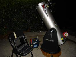
Introduction

This tutorial will cover planetary imaging and image processing, describing the steps and methods I use to process an image taken with a webcam such as the ToUcam. It is not intended to cover the actual capturing of the avi, though factors that influence good data capture and a guide to capture settings will be discussed.

The most important factor in getting any high quality image is the seeing. If the data is great to begin with, then very little processing is actually required to end up with a great image. However most of us don’t have the luxury of imaging in an area with no jetstream, or in an area where the planet is directly overhead. Through experience I’ve found that when the conditions are less than ideal, a better result can be achieved through the processing steps outlined below.

It’s worth noting now that there are many ways to process an avi, and this routine may not be for everyone. Sometimes the extra effort is not really worth it, and at other times it may produce a 5%-30% better image. For me, any improvement in the final result is worth the extra effort as I try and extract the most out of my equipment.

It’s also worth noting that how a final image looks is a very personal preference. Colour balance, and the amount of contrast and sharpening are settings that you have control over, and you decide how the final image looks. Some people prefer a “natural” looking image with smooth detail and little sharpening. Other people prefer to increase contrast and sharpen the image more to enhance the finer detail and make it more visible. As I said, it’s personal preference and you’ll need to modify the steps below to suit your tastes.

All of my imaging is done with modest affordable equipment. I use a 10” GSO dob (newtonian reflector) on an EQ platform by Round Table Platforms . The focal length is 1250mm. I use a ToUcam webcam as my capture device, with a 5x Powermate for increased focal length and image scale. The picture below shows my imaging setup.

Click to Enlarge My imaging setup

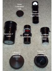
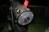
Factors that Influence the Data you Get

There are many factors that influence the quality of the data you capture. You should ensure that you do all you can to minimise these factors and give yourself the best possible chance to capture good data.

Seeing

Seeing is King. If the seeing is very good, you’ll most likely get a very good image as long as you have the basics in order (collimation and cooling). Conversely, even if your collimation is perfect and the scope is at ambient temperature, if the seeing is no good, you just won’t get a good image.
Seeing is a very tricky thing to predict and analyse. The jetstream maps give an indication of the speed of high altitude winds over your area. If there’s a fast jetstream above you, it’s likely that the seeing will be pretty ordinary. If there’s no jetstream above you, you have a better chance of getting good seeing. The left image below shows a typical jetstream map during Winter in Australia.

You can also try judging the seeing by the twinkling of the stars (naked eye). The more they are twinkling, the more likely it is that there’s turbulence in the atmosphere that will negatively affect the seeing. It’s not an exact science though so the best approach is to put a high power eyepiece in and check it out for yourself. If the view is stable and you can see reasonable detail, then put the webcam in and start capturing!

Collimation

Collimation is a basic skill that every telescope owner needs to master. If the collimation is not right, the image will always appear soft. You must learn how to collimate your scope!

If you’re doing high resolution imaging, you should check your collimation before every imaging session and get it as close to perfect as possible. I’m not going to discuss how to collimate as there’s a thousand resources on the web that go into great detail, but make sure you learn how to do it. If you’re not sure you’ve got it right, get some advice on the IceInSpace Forums, or find another forum member that lives nearby and ask them to help you.

The middle image below (courtesy Tom Hole) shows an array of collimation tools.

Cooling

If the mirror temperature is not close to ambient, you’ll get a boundary layer of air sitting on top of the mirror which will distort your image and give the appearance of bad seeing. Often, tube currents and the boundary layer are misinterpreted as bad seeing. To help eliminate those factors, you should passively or actively cool your mirror down to ambient temperature.

At a very minimum, take your scope out hours before you plan to begin imaging to allow the mirror to cool to ambient. If the ambient temperature is also dropping, the mirror will never catch up. That’s when you should think about actively cooling your mirror by using a cooling fan and/or peltier coolers. The image on the right below shows the results of my own cooling fan project. Hopefully another article will come in the future which describes how to do this.

Click to Enlarge Jetstream map		Click to Enlarge Collimation Tools		Click to Enlarge Cooling Fan

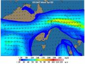
Altitude

Generally you have a much better chance of getting good data if you’re capturing when the image is higher in the sky. When the object is higher, you’re looking through  less “junk” in the atmosphere and there’ll be less atmospheric distortion of your image.

Sometimes we don’t have a choice, as depending on where you live, the planet might only reach 35° altitude. In those cases, you’ll always be struggling. Ideally, the planet should be above 50°. The higher the better!

Capture Device

This article is mainly targeted to those using cheap webcams like the ToUcam to do imaging, but it also relevant for those using high end webcams like the Lumenera, DMK or PGR cameras. Some factors that influence the choice of capture device:

Frame Rate and Compression
The Toucam (840k and 900nc) is a USB1.1 device, so it has to compress the data to shove it down the pipe as fast as you are capturing. This compression leads to artefacts and loss and detail. Ideally you don’t want any compression, but you also have to weigh that up against using a fast framerate to capture as many frames as possible trying to get those brief moments of steady seeing.
I’d suggest using 5fps in great seeing, and 10fps any other time. At 5fps, you’re capturing less frames, but there’ll be less compression so at least you’ll have the best quality data to work with. At 10fps, there’s more compression, but if the seeing is only average, you want to capture more frames in the hope that you’ll find more sharp frames amongst the bad ones.
The high-end webcams avoid this problem because they’re USB2 or firewire interface to the computer. This means they can transfer the data as fast as you can capture it, without any compression. So you can capture at 30fps with no compression, which gives you a much greater chance of finding sharp frames even when the seeing is not good.

Colour versus Mono
The ToUcam is a colour camera, so are some of the high end cameras like the LU075C and DMK21F04. This means they have a colour CCD chip in a bayer filter configuration, where 50% of the sensor captures green wavelength light, 25% captures red and 25% captures blue. This means you’re not getting the whole 640x480 resolution in each colour channel.
A mono CCD chip on the other hand, in combination with Red, Green and Blue filters that allow only the Red, Green and Blue wavelengths of light through, use the whole 640x480 resolution to capture each colour channel. You also have the option to change capture settings and refocus each colour channel as you capture it.
So using a monochrome camera like the LU075 or DMK21AF04 gives the best resolution, at the expense of cost and convenience. They are more expensive to buy, and you need to buy a filter wheel and RGB filters as well. You also have the added frustrations of changing filters, refocusing and recapturing, all within a short capture window.
What you decide to get, should be based on your budget, skills and frustration threshold. :) However the best results will be achieved with a monochrome, high-speed camera.

Click to Enlarge ToUcam 840k		Click to Enlarge DMK21AF04

Capture Settings

As long as the raw data you’re capturing isn’t too bright (overexposed) or too dark (underexposed), there’s not a lot that can go wrong here.

Processing

The final step, and that’s where this tutorial comes in! :)

All of those factors above can and will play a part in the quality of your image - so I'd recommend doing all you can to understand and address each of them.

Capturing the Data

The capture settings you use will vary greatly depending on factors such as:

• The telescope and type of telescope
• The focal length you are working at (including barlows/extensions)
• The frame rate you use
• What object you are imaging
• How bright the image is
• The local transparency (clouds, haze, fog, dust, etc)

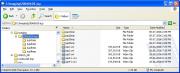
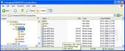
As such, there’s no “ideal” settings. You have to experiment to find the best combination for your scope and camera and local conditions.

As a general guide, if you’re using K3CCDTools to capture, have the white level meter somewhere between 210 to 230. This ensures you have sufficient exposure to capture the dim areas, without overexposing and burning out the bright areas.

Don’t be afraid of gain, even up to 50% or more if needed. A higher gain will make your image grainier, but if you can capture enough frames to stack you’ll be able to smooth it out.

Don’t be afraid of gamma. I capture with 45-50% gamma, always. It makes the image look washed out during capture, but it ensures you’re capturing enough dynamic range in the dim areas. I reduce the gamma in post processing which enhances the contrast and reveals more detail.

Check focus regularly! The focal point can change as the image gets higher in the sky, and as your mirror changes shape as the temperature drops. Some people check focus between each avi! I check it after every 2 or 3 avi’s. If you can’t get that snap focus you’re searching for, it’s likely that seeing and/or tube currents are the culprits.

The total length of time you should capture each avi for varies depending on the object you’re imaging and it’s rotation speed. As a general rule, you can image Jupiter for 2 minutes, Saturn for 5 minutes or more (unless there’s a storm you’re trying to image), Mars for 4 minutes and the Moon for several minutes. The length of time also is determined by your effective focal length, as the longer the focal length you’re working at, the faster the rotation will be visible.

Processing the Data

Ok, so you’ve got an avi or two. The old routine would involve simply running that avi through registax, aligning/stacking and wavelet processing to get the final result. That’s still a valid way to process, but I’ve found that the extra steps below help to get the most out of the data you’ve got.

Software

You’ll need some extra software to follow this processing routine. You can download the software by clicking on the links below.

Virtual Dub (homepage)
Used to convert the avi into a set of bitmap (BMP) files. The bitmap files are required because the programs in the following steps work on bitmap files, not videos.

PPMCentre (homepage)
Windows command-line tool used to crop, centre and rank the BMP files.

PPMCentre Front End (PCFE download)
A separate frontend-GUI used to set the desired options and run ppmcentre. Takes the fear factor away from those people who are command-line challenged :)

RGBSplit (download)
A program used to split the BMP files into their Red, Green and Blue channels.

Registax (homepage)
A program used to align, optimise, stack and process each set of Red, Green and Blue bitmaps.

AstraImage (homepage)
A program used to perform deconvolution on the resulting Red, Green and Blue channel images, and recombine them back into a colour image.

Photoshop CS (hompage)
Used for final adjustments of colour balance, levels, contrast, sharpness and preparation for web posting.

Processing Steps

Directory Structure

Create a directory such as e:\imaging. All of the required software should go there.
For each imaging session, create a sub-directory with the date and subject as the name. For example, e:\imaging\20060628-jup.

Your avi’s should be captured (or moved) into that directory. I name them like “jup1.avi”, “jup2.avi”, and where I’ve had to capture multiple avi’s in the same capture window, append a sequence such as “jup3-1.avi”, “jup3-2.avi”.

In that directory, I now create sub-directories for each of the avi’s where the bitmap files will be stored. So I’ll end up with e:\imaging\20060628\jup1bmp, e:\imaging\20060628\jup2bmp and so on.

Click to Enlarge Directory Structure

We’re now ready to start processing.

Saving the AVI as BMP’s using VirtualDub

This step is required because ppmcentre and RGBSplit work on BMP files, not AVI files. It can be done in batch, or individually. At the moment, I pass each AVI through VirtualDub as soon as I’ve finished capturing it. By the time VirtualDub has finished (approximately 2 minutes), I’m ready to capture the next one.

Using VirtualDub, open the avi. If you have multiple avi’s over the same capture period (2 minutes), combine them by using “Append AVI” after opening the initial one. I use the right and left arrows to move through the avi and delete any obviously bad frames blurred due to a bad moment of seeing, bumping the scope, or the planet drifting off the edge of the frame due to inaccurate tracking.

Then go to File -> Save Image Sequence, and save as a set of BMP files into your BMP directory. See example below.

Click to Enlarge Virtual Dub save BMP's

Run the BMPs through PPMCentre

Using PPMCentre has 3 main advantages:

1. Centering the planet in the middle of the frame
   Great for those with inaccurate tracking because registax seems to handle aligning much better when the tracking is accurate. It also makes registax faster.
2. Cropping
   Cropping to 400x400 (more or less) is good because it makes the whole processing in registax much faster.
3. Ranking
   If you use the qestimator and renumber functions, it basically does a "gradient" analysis on each frame, and then renumbers them to rank them in best to worst order. Now when you drag them into registax, frame 0000 is the best. When you align in registax, you can choose the alignment feature on the best frame, which generally means registax should align and rank the frames much more accurately.

By default, it will simply centre the object in the middle of the frame. The extra command line parameters are for additional features such cropping and ranking. You can see all the command line options and what they do by visiting the ppmcentre homepage.

To run ppmcentre, you can either run it directly from a dos window, or use the handy GUI written by Adam Bialek.

To run it from DOS, open up a dos window (Start -> Run -> “cmd”), and change directory to your imaging directory by typing “cd e:\imaging”. Run ppmcentre on one of your bitmap directories by typing the following:

ppmcentre -width=400 -height=400 -cutx=400 -cuty=400 -overwrite -qestimator -renumber e:/imaging/20060628-jup/jup2bmp

You can repeat this for all of your BMP directories.

To run it from the frontend GUI, choose the BMP folder(s) you want to process, check and set the command line options you want to use, and hit process!

I overwrite my original bitmaps with the ppmcentre-processed ones. You can choose to write the processed bitmaps out to a new directory. It’s up to you.

Click to Enlarge PPMCentre DOS version		Click to Enlarge PCFE (PPMCentre Front End)

Splitting the BMP’s into R/G/B channels

There’s nothing stopping you from taking the resulting BMP’s from ppmcentre and feeding them straight into registax now, rather than go through the extra step of splitting them into r/g/b channels. In fact, this is exactly what I do after each imaging session, as it allows me to get a feel for the quality of each avi and determine which of the avi’s I captured have the best quality, sharpest data.

I’ll drag the BMP’s from windows explorer into registax, and process it like any other avi or set of bitmaps (align/reference frame/optimise/stack/wavelets). I spent as little time as possible here, as I’m just using to judge the quality of the avi. I save the resulting image as a “quick” run, and repeat this for all “sets” captured during that session. If some avi’s are obviously bad, I delete them and their bitmaps. If some avi’s are obviously better, these are the ones I’ll spend the most time on processing, and they’ll receive the lengthier processing of splitting into R/G/B channels and separate processing. If I want to create an animation, I’ll process all avi’s using the methods below so that all images that make up the animation look and feel the same.

So now you’ve decided to split the BMP’s that ppmcentre produced, into their red, green and blue channels. The reason I choose to do this, is because:

1. It allows different processing on each channel. That is, you might want to perform some noise reduction on the blue channel only, or you might want to sharpen the red channel more than the others.
2. Registax appears to find it easier align and stack when working on individual colour channels, rather than a colour frame. In a colour frame, misaligned colour channels due to atmospheric dispertion tend to confuse registax and you can end up with artefacts in your image after stacking.

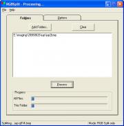
To split the BMP’s into their red, green and blue channels, use the GUI developed by Adam Bialek. Simply add the folder name(s) that contain the BMP’s, set the parameters and hit Process.

You’ll end up with 3 sub-directories (Red, Green, Blue), each containing the respective red, green and blue channels from the original colour bitmap.

If in doubt, read the walkthrough documentation for RGBSplit.

Click to Enlarge RGBSplit		Click to Enlarge Directory structure after ppmcentre + RGBSplit

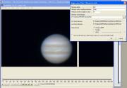
Registax Processing

Everyone should be familiar with registax already, but I’ve found that most people use it in slightly different ways as there’s so many settings that can be changed. In this section I’ll describe how I use registax to produce a stacked, processed image of each colour channel from the bitmaps that have already been passed through ppmcentre and then split into R/G/B channels by RGBSplit.

Open up registax, and then back in Windows Explorer, select all of the bitmaps in your “Red” directory by clicking Ctrl-A. Drag them onto the registax window and let them go.

Alignment

If you used the qestimator and renumber options in ppmcentre, then find the frame marked “jup1-q0000” for example. That will be the best quality frame as determined by ppmcentre. Put the focus on the frame selector at the bottom, and use your left and right arrows to scroll through the frames to find frame q0000.

You can see in the screenshot the settings I use (that is, gradient algorithm). You can ignore the cutoff % for now, as we change this manually later.

Click to Enlarge Size and position of alignment window

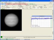
I use a 128px alignment window, and select a feature of interest that you want to be sharp – for example, the GRS, a moon transit shadow, etc. Click align, and wait for it to get to 100%.

Ideally, you should end up with a graph that slopes up to the right, starting low on the left. The best quality frames are on the left end, and the worst quality are on the right. Here’s when we decide to drop some frames from further processing. Using the frame select slider down the bottom, drag it left or right to a point where the graph starts rising up sharply. Everything to the left of the slider is kept, everything to the right is thrown away. In this example below, because the seeing was quite good, the quality of most of the frames is high so i've decided to keep almost all of them.

Once you’re happy, hit Limit to move to the Optimise tab.

Click to Enlarge After alignment, limiting frames.

Optimise

The first thing I do when reaching this tab, is to create a reference frame. This gives the optimiser a “better” frame in which to compare all other frames against. I leave the default of 50 frames, and hit “Create Reference Frame”. Once you end up in the wavelets tab and click “ok” past the information message, I set wavelet 3 to 10.5 and wavelet 4 to 15.2, and that’s it. You can save those wavelet settings by clicking “Save Settings” and call it something like “mild”. Next time, you just use “Load Settings” and choose “mild”, and it will apply those settings. See the left image below for how it looks.

Press “Continue” to go back to the Optimise Tab.

Click “Optimise” and registax will usually make 3 passes through the frames, and the resulting graph will hopefully be sloping up from low on the left to higher on the right.  See the right image below for how it looks.

Now move to the Stack tab.

Click to Enlarge Create Reference Frame wavelet settings		Click to Enlarge Shape of the graph after Optimise

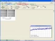
Stack

Click the “Stack Graph” tab on the right hand side. This is where you choose how many frames you want to stack. The choice is a fairly important one, as if you stack too few frames, the image will be noisy and grainy. If you stack too many, you may end up stacking bad quality frames in with good ones, which will soften the image and it’ll be less sharp after applying wavelets. The left image below shows the stack graph.

You can drag the vertical slider down or the horizontal slider to the left to restrict the number of frames you want to stack. Everything above the horizontal line and to the right of the vertical line will get thrown away. The number of frames that will be stacked is shown in the status bar at the bottom (n=161 seen in the left screenshot below).

How many you should stack depends on the quality of the data and how many frames in total you’ve got to choose from. I tend to stack between 100 to 160 frames, where I’ve captured a total of about 600 using 5fps for 120 seconds on Jupiter (for example).

In general, I believe it’s better to stack less GOOD frames than more BAD frames. Try and drag the vertical slider down to the point where the graph starts rising up too high on the right.

Click Stack to begin, and when it’s finished you’ll see the resulting stacked image before any further processing (right screenshot below). Now move to the wavelets tab.

Click to Enlarge Stackgraph, deciding how many frames to stack		Click to Enlarge The result after stacking

Wavelets

Now to the fun part.. Wavelet processing is mostly black magic to me. There’s a thousand sites on the internet where you can read about wavelets, what they are and how they work, but in our context, I think it’s enough to know that it’s a way to reduce noise and extract detail from an image.

I apply the following wavelets to the image: 3 @ 10.5, 4 @ 15.2, 5 @ 16.5. I’ve got those settings saved, so when I come into the wavelets tab I just load settings, and it’s done.

Click “Save Image” on the right hand side, and save as a TIFF. I call it something like “jup2-red.tif”.

Click to Enlarge The red channel after wavelets have been applied

That’s the red channel done for now! I close registax and re-open it, and now I select all the bitmaps from the Green folder, and drag them into registax. I repeat exactly the same process, and save the image as “jup2-green.gif”. Rinse and repeat for the blue channel bitmaps.

Our time with registax is done, now to process those images in AstraImage!

AstraImage Processing

I use AstraImage to perform deconvolution on each of the images saved from registax, before recombining them back into a colour image.

Deconvolution is an iterative image processing filter that uses Fourier transform mathematics in an attempt to reverse the optical distortion that takes place in a telescope, thus creating a clearer image.

Again, it’s mostly black magic to me but through experimentation I’ve found some processing that helps to reveal detail and sharpen the image.

Open each of your images saved from registax (jup2-red, jup2-green and jup2-blue).

Click to Enlarge After opening the 3 channels in AstraImage

At this stage, they are classified as colour images (even though they single channels), so they have to be converted to greyscale. On each image, click “Process -> Greyscale”. It does an implicit histostretch on the image so you’ll usually end up with a brighter image after this step.

I now usually do a LR deconvolution on each of the greyscale images, with the iterations at 7 and the curve radius of 1.4.

Click to Enlarge After greyscale, showing settings for LR deconvolution

The values you use here depend on the quality of the data, how sharp it already is, and how many frames you stacked in registax. It’s really trial and error to find the right settings for each circumstance so I suggest you simply experiment.. try a smaller curve radius, try less iterations, try more, etc.

Ideally you’re after a resulting image that has revealed more detail without being oversharpened. You can tell if you’re oversharpening because the features start looking bloated and you’ll start getting hard ringing around the edge of the planet.

The image on the left below shows the result after all 3 channels have had LR deconvolution applied.

You can also try ME deconvolution, VC deconvolution and/or FFT filtering. There’s a lot of different settings you can try – as I said, just experiment and find what works for you.

We now want to recombine the individual channels back into a colour image. You do this by clicking on “Process -> Recombine”. In the dialog, for the red dropdown you want to choose the image that had LR deconvolution performed on the Red channel. Same for the other 2 channels. The easiest way is to rename the images after they’ve had LR deconvolution applied – do this by clicking “Edit -> Image Title”, and call it something like “LR-red”, “LR-green”, and so on. That way, in the dropdowns you can find the correct images to recombine.

Once you’ve selected them in the dropdown, click “Update”. You now need to align the colour channels before clicking apply, as they can be misaligned by a few pixels due to atmospheric dispersion. The image on the right below shows the recombined image before being realigned.

Click to Enlarge All 3 channels after LR deconvolution		Click to Enlarge Recombining, see the blue rim on the left and top

What you’re looking for here, is a red or blue rim around the planet in one direction only. For me, blue usually needs to be moved down and to the right, and red usually needs to be moved up and to the left. But not always – it depends on the altitude that the image was captured at, as the higher the altitude, the less atmospheric dispertion. You can try zooming in to get a better view, but the preview window does leave a lot to be desired.

In this example, blue had to be moved down 1 pixel and to the right 1 pixel. Red had to be moved up (-1) 1 pixel. You can see from the preview window (image on the left) that there’s now no blue or red rim and the colour channels are nicely aligned.

You can now hit apply and see the recombined colour image (middle image below).

Because I capture with high gamma, now I want to reduce the gamma to give greater depth and contrast. Click on “Scale->Brightness and Gamma”. I reduce to 0.7, click apply. You can see the image after gamma reduction on the right below.

Save the image as TIFF, and take it into Photoshop!

Click to Enlarge Showing the preview realigning the red and blue channels		Click to Enlarge After recombined into a colour image		Click to Enlarge After gamma reduced to 0.7

Photoshop Processing

I use photoshop to do any final adjustments to the image, and also to save it for the web. The adjustments may include levels or curves adjustment, saturation, colour balance and final unsharp mask. What final adjustments are needed depend mostly on personal taste, so the process outlined here should be taken as a guide only.

I open the TIFF, and use the circle selection tool with a feather of 35px to select the inside edge of the planet. I create a new curves layer, and adjust the curves down as shown in the left image below, to give more colour depth and contrast.

The left image below shows the selection, and the right image shows the curves used.

Click to Enlarge Showing the selection		Click to Enlarge Showing the curves

If required, I create new layers to adjust colour balance or saturation to taste.

I then select the background layer again, and apply an unsharp mask. The radius and pixel size I use depends on how much sharpening is required. Sometimes this step introduces too much grain or artefacts from oversharpening, so use it in moderation. The resulting image is the left one below.

And that’s basically it.

I now add the “fluff” around the image for presentation. I save the image with the layers as a PSD file incase I want to edit it later, and I save it as TIFF (with no layers) as well.
For web presentation I do “Save for Web” and reduce the jpeg quality to save it under 150k or 100k, depending on the forum rules where it needs to be posted. The final image is seen on the right below.

Click to Enlarge After unsharp mask		Click to Enlarge Final image!

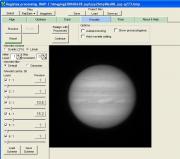
Processing with Moons in the Frame

If your avi has satellites in the frames as well, it’s worth more time again to process the moons separately from the main planet. Aligning on a feature on the planet will make the planet sharp, but the moon part of the frame may not be sharp. Also, if the moon moves slightly during the capture time then it can end up elongated and not round.

To process the moons separately, most times it’s probably not worth the extra effort of processing the moon in red, green and blue channels. Just take the colour bitmaps from ppmcentre, and feed them into registax.

Find a sharp frame where the moon is nice and round, and use a 32px alignment window to select it. Go through the same registax processing outlined above, and save the image as a TIFF, for example “jup1-ganymede.tif”.

The image on the left below shows the moon being selected in the alignment tab in registax.

Open the moon TIFF, and the processed planet TIFF in photoshop. The planet TIFF will be your master image. On the moon image, use the rectangle select tool to select the moon and part of the planet (to help with aligning), and copy the selection. Go back to the planet image and paste the selection as a new layer. Use the move tool to line up the pasted moon layer over the top of the original.

Once it’s lined up, select the area of the moon layer that covered the planet, and press delete to delete it from that layer. It leaves the moon on its own in the new layer, on top of the planet picture on the bottom layer.

The image on the right below shows this process, and shows the benefit of separate processing as the moon on the final image is sharper with better colour detail. 

Click to Enlarge Moon selection area in Registax		Click to Enlarge Showing the processed moon layer over the processed planet image

Some Before and After Examples

Here are a few examples of some images that I’ve offered to reprocess for the imager, because I’ve seen that the data is good quality but the processing didn’t bring out the best in it.

• The top row shows an image by IceInSpace Forum member John K, taken on the 17th April 2006 with a JMI NGT 12.5" f/5 w/Torus Optics, a 5x powermate and a NexImage webcam. The original is on the left, my reprocessed version is on the right.
• The second and third rows show an image by IceInSpace Forum member Gary Beal, taken on the 17th May 2006 with a 10” newt, a 5x powermate and a ToUcam webcam. The originals are on the left, my reprocessed versions are on the right.
• The fourth row shows an image by IceInSpace Forum member Hitchhiker, taken on the 12th June 2006 with a Meade 10" LX200GPS + 2.5X Powermate + LPI. The image shows the originals on the left and my reprocessed versions on the right.

My reprocessed versions were done using the exact methods outlined above.

Click to Enlarge John K original image		Click to Enlarge John K reprocessed
Click to Enlarge Gary Beal original image		Click to Enlarge Gary Beal reprocessed
Click to Enlarge Gary Beal original image		Click to Enlarge Gary Beal reprocessed
Click to Enlarge Adam Bialek originals and reprocessed

Processing Examples

Here are a few of my animations taken between February and June 2006, processed using the methods outlined above. The animations were created in Jasc Software Animation Shop 3. All the animations are GIF files, and are between 300-600kb.

Animations

• 25th February 2006
• 12th March 2006
• 26th March 2006
• 30th March 2006
• 4th May 2006
• 25th May 2006
• 12th June 2006
• 14th June 2006
• 16th June 2006

Conclusion

As mentioned at the start of the article, there are a bunch of different ways to process an avi. My method may not be for you, but it may be worth giving a try. It’s a longer process than most people go through, but if it gives an even 5-10% better image, then it’s worth the extra hassle.

I hope this article helps you to produce better images. I welcome your feedback.

Article by Mike Salway (iceman). Discuss this article on the IceInSpace Forum.